

how to find the coefficient of determination
10.6: The Coefficient of Determination
- Page ID
- 553
Learning Objectives
- To learn what the coefficient of determination is, how to compute it, and what it tells us about the relationship between two variables \(x\) and \(y\).
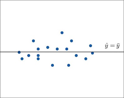
If the scatter diagram of a set up of \((ten,y)\) pairs shows neither an upward or downwards trend, then the horizontal line \(\hat{y} =\overline{y}\) fits information technology well, every bit illustrated in Effigy \(\PageIndex{ane}\). The lack of any upward or downward trend means that when an element of the population is selected at random, knowing the value of the measurement \(x\) for that element is not helpful in predicting the value of the measurement \(y\).
If the scatter diagram shows a linear trend upwardly or down and then it is useful to compute the least squares regression line
\[\lid{y} =\chapeau{β}_1x+\hat{β}_0\]
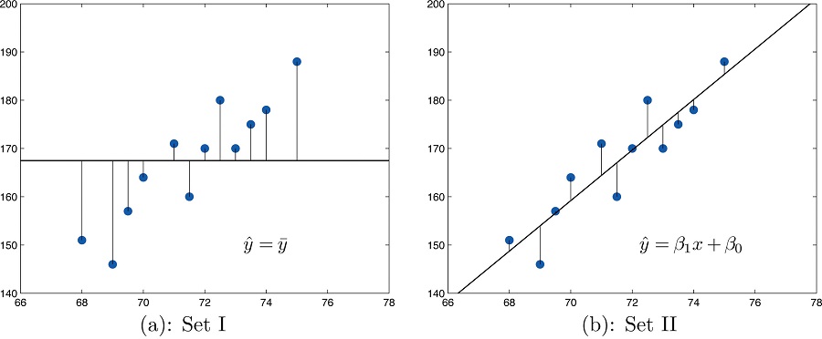
and utilize it in predicting \(y\). Figure \(\PageIndex{2}\) illustrates this. In each panel we have plotted the height and weight information of Section x.i. This is the same scatter plot as Figure \(\PageIndex{2}\), with the average value line \(\hat{y} =\overline{y}\) superimposed on information technology in the left console and the least squares regression line imposed on it in the right panel. The errors are indicated graphically by the vertical line segments.
The sum of the squared errors computed for the regression line, \(SSE\), is smaller than the sum of the squared errors computed for any other line. In detail information technology is less than the sum of the squared errors computed using the line \(\hat{y}=\overline{y}\), which sum is actually the number \(SS_{yy}\) that we have seen several times already. A measure out of how useful it is to employ the regression equation for prediction of \(y\) is how much smaller \(SSE\) is than \(SS_{yy}\). In particular, the proportion of the sum of the squared errors for the line \(\hat{y} =\overline{y}\) that is eliminated past going over to the least squares regression line is
\[\dfrac{SS_{yy}−SSE}{SS_{yy}}=\dfrac{SS_{yy}}{SS_{yy}}−\dfrac{SSE}{SS_{yy}}=1−\dfrac{SSE}{SS_{yy}}\]
Nosotros can think of \(SSE/SS_{yy}\) as the proportion of the variability in \(y\) that cannot be accounted for by the linear human relationship between \(x\) and \(y\), since it is still at that place even when \(x\) is taken into account in the best mode possible (using the least squares regression line; remember that \(SSE\) is the smallest the sum of the squared errors tin can be for any line). Seen in this light, the coefficient of determination, the complementary proportion of the variability in \(y\), is the proportion of the variability in all the \(y\) measurements that is accounted for by the linear relationship between \(x\) and \(y\).
In the context of linear regression the coefficient of determination is always the square of the correlation coefficient \(r\) discussed in Section x.2. Thus the coefficient of conclusion is denoted \(r^ii\), and we have two additional formulas for computing it.
Definition: coefficient of determination
The coefficient of determination of a collection of \((10,y)\) pairs is the number \(r^2\) computed by whatever of the post-obit three expressions:
\[r^2=\dfrac{SS_{yy}−SSE}{SS_{yy}}=\dfrac{SS^2_{xy}}{SS_{xx}SS_{yy}}=\hat{β}_1 \dfrac{SS_{xy}}{SS_{yy}}\]
It measures the proportion of the variability in \(y\) that is accounted for past the linear human relationship between \(x\) and \(y\).
If the correlation coefficient \(r\) is already known and then the coefficient of determination tin be computed but by squaring \(r\), equally the note indicates, \(r^2=(r)^2\).
Example \(\PageIndex{one}\)
The value of used vehicles of the make and model discussed in "Example x.4.2" in Section ten.four varies widely. The most expensive auto in the sample in Table 10.4.iii has value \(\$30,500\), which is near half again every bit much as the least expensive one, which is worth \(\$20,400\). Notice the proportion of the variability in value that is accounted for past the linear relationship between age and value.
Solution:
The proportion of the variability in value \(y\) that is accounted for past the linear relationship between it and age \(10\) is given past the coefficient of conclusion, \(r^2\). Since the correlation coefficient \(r\) was already computed in "Case ten.4.two" in Section 10.four equally
\[r=-0.819\\ r^2=(-0.819)2=0.671\]
About \(67\%\) of the variability in the value of this vehicle can be explained by its age.
Example \(\PageIndex{2}\)
Employ each of the three formulas for the coefficient of determination to compute its value for the instance of ages and values of vehicles.
Solution:
In "Example ten.iv.2" in Department 10.4 we computed the verbal values
\[SS_{twenty}=fourteen\\ SS_{xy}=-28.7\\ SS_{yy}=87.781\\ \hat{\beta _1}=-two.05\]
In "Case ten.4.four" in Section 10.4 nosotros computed the exact value
\[SSE=28.946\]
Inserting these values into the formulas in the definition, ane later on the other, gives
\[r^2=\dfrac{SS_{yy}−SSE}{SS_{yy}}=\dfrac{87.781−28.946}{87.781}=0.6702475479\]
\[r^2= \dfrac{SS^2_{xy}}{SS_{xx}SS_{yy}}=\dfrac{(−28.7)^2}{(14)(87.781)}=0.6702475479\]
\[r^ii=\hat{β}_1 \dfrac{SS_{xy}}{SS_{yy}}=−2.05\dfrac{−28.vii}{87.781}=0.6702475479\]which rounds to \(0.670\). The discrepancy between the value hither and in the previous case is because a rounded value of \(r\) from "Instance 10.4.two" was used there. The actual value of \(r\) before rounding is \(0.8186864772\), which when squared gives the value for \(r^2\) obtained here.
The coefficient of decision \(r^2\) tin always be computed past squaring the correlation coefficient \(r\) if it is known. Whatever one of the defining formulas can also be used. Typically 1 would make the choice based on which quantities have already been computed. What should exist avoided is trying to compute \(r\) by taking the square root of \(r^two\), if information technology is already known, since it is piece of cake to make a sign error this way. To see what can go wrong, suppose \(r^two=0.64\). Taking the foursquare root of a positive number with any computing device volition e'er return a positive result. The square root of \(0.64\) is \(0.8\). However, the bodily value of \(r\) might be the negative number \(-0.8\).
Key Takeaway
- The coefficient of determination \(r^2\) estimates the proportion of the variability in the variable \(y\) that is explained by the linear relationship between \(y\) and the variable \(x\).
- In that location are several formulas for computing \(r^2\). The choice of which one to use tin be based on which quantities have already been computed so far.
Source: https://stats.libretexts.org/Bookshelves/Introductory_Statistics/Book:_Introductory_Statistics_%28Shafer_and_Zhang%29/10:_Correlation_and_Regression/10.06:_The_Coefficient_of_Determination
Posted by: knightwoust1984.blogspot.com
0 Response to "how to find the coefficient of determination"
Post a Comment